Venturi Mass Flow Measurement
After completing a design, it is important to be able to measure whether the expected performance has been met and if not, where improvements have to be made. In my case, i had to measure whether a 3D-printed nozzle did perform as desired and actually give the calculated mass flow.
Mass flow is not a quantity than can be directly measured. The way to do it is to calculate it from the flow speed $c$ as
\[\begin{equation} \dot{m} = \rho c A \end{equation}\]The density is usually known from temperature and pressure with the ideal gas law and the flow cross section can be measured as well.
In order to measure the flow speed, multiple solutions exist, ranging from the hot wire anemometer where flow speed is correlated with the heat flux from a heated wire in the flow, to optical speed measurement of suspended particles. In some cases, it is also possible to measure flow speed from the vortex shedding frequency on a rod in the stream. In my case i wanted a simple solution without much electronics that is why i decided to build a Venturi flowmeter.
Venturi Flowmeter Principle
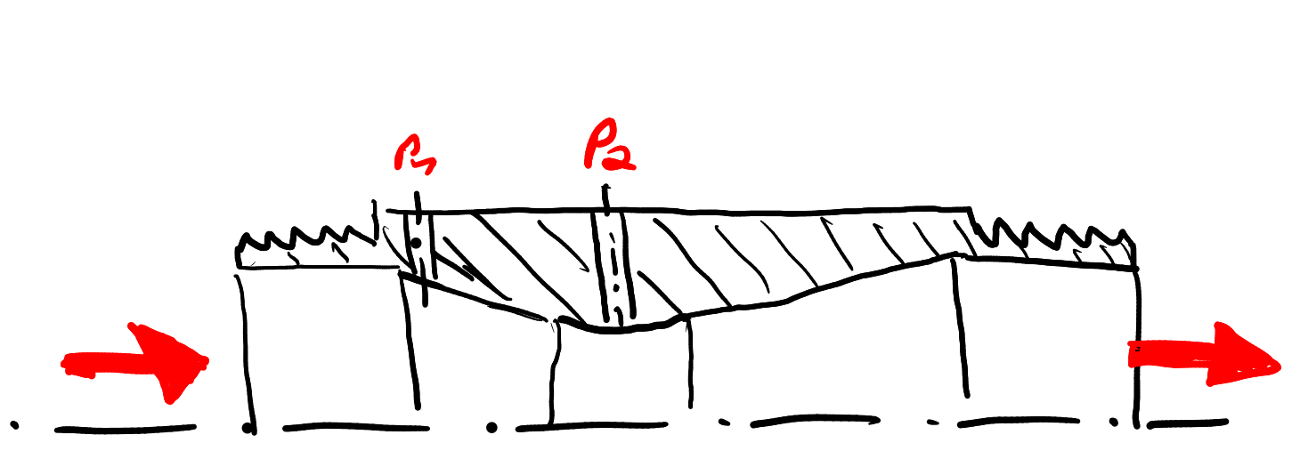
The Venturi Flowmeter consists of a converging-diverging nozzle which accelerates the flow and a differential pressure measurement that monitors the accompanying pressure drop.
If we use Bernoullis equation for a stationary, incompressible, adiabatic and isentropic flow, the following relation between pressure and velocity can be derived:
\[\begin{equation} p_t = p + \frac{\rho}{2} c^2 \end{equation}\]which is constant along a streamline.
Applying this to a point on the streamline before the constriction (indexed with 1) and a point on the same streamline directly at the throat (indexed with 2) gives the following relation:
\[\begin{equation} p_1 + \frac{\rho}{2} c_1^2 = p_2 + \frac{\rho}{2} c_2^2 \end{equation}\]From the conservation of mass and incompressibility, another relation can be derived:
\[\begin{equation} c_1 = c_2 \frac{A_2}{A_1} \end{equation}\]These two can be combined to find:
\[\begin{equation} c_1 = \sqrt{2 \frac{p_1-p_2}{\rho \left(\frac{A_1^2}{A_2^2} - 1\right)}} \end{equation}\]This means that the flow speed the throat can be calculated from the pressure difference before the orifice and at the throat. The absolute pressure must be known as well. For the accuracy that i required, this is not a big problem. I just assume $p_1$ to be known (read off of the compressor), just as i already did in the previous case in order to calculate the density from the ideal gas law (mass flow calculation).
The difference is easily measured by a differential pressure transducer such as the NXP MPX5500. This device works by measuring the displacement of a membrane with the two different pressure that are to be compared with the help of a piezoelectric sensing element. A voltage that is directly proportional to the pressure difference is produced at the output pin of the sensor.
Behind the throat, the flow is returned to the normal pressure and cross section. Here, the cone half angle is quite narrow, as this diffuser is prone to flow separation. In that case, the total pressure would not be recovered because of losses and the pressure behind the measurement point is reduced.
The Venturi nozzle i created can be found unter this thingiverse link. It is meant to be inserted into a piece of aquarium hose with $\pu{4 mm}$ ID, $\pu{6 mm}$ OD. From the Venturi dimensions $r_1 = \pu{2 mm}$, $r_2 = \pu{0.9 mm}$, the equation for low Mach speeds is $c_1= \pu{84.4 m/s^2} \sqrt{\frac{\Delta p}{p_1}}$. The measurement holes are spaced to fit the MPX5500 sensor, which is inserted and sealed by two pieces of the same tubing.
For my test i inserted this Venturi nozzle into a line, with a compressor running at $\pu{5 bars}$ on one end and a flow constricting nozzle at the other end. I measured a pressure drop of around $\pu{1.1 bar}$, which gives a velocity of $c_1 \approx \pu{40 m/s}$. The hereby calculated mass flow of $\dot{m} \approx \pu{3 g/s}$ is also in the same ballpark range as the specification of my compressor, which is $\pu{23 l/min}$, so $\pu{2.3g/s}$ at $\pu{5 bar}$ and $\pu{290 K}$.
Going Incompressible
We have however assumed an incompressible flow while using air as a medium - which is definitely compressible. Whether compressible effects are of relevance can be checked by calculating the Mach number.
\[\begin{equation} \Mach^2 = \frac{c^2}{\gamma R T} \end{equation}\]If it is smaller than about $0.3$, the incompressible assumption is usually good enough.
It can of course not be calculated exactly without knowledge of the actual flow speed, but we can still check the Mach number attained with the incompressible calculation for its validity.
In my case, the measured Mach number was around $0.1$. However at point $2$, it is higher by a factor of $\frac{A_1}{A_2}$, so around $0.5$, above the range where compressible effects are dominant.
If the Mach number approaches one, the density is not anymore a constant. This changes a lot of things. Previously, we were able to remove the density from both sides of the mass conservation equation (turning it into a conservation of volumetric flow), as it was the same for both points. This is not anymore possible.
As we now have two density values, we also need an additional equation to close the system. This is the conservation of energy, which can be written in terms of the total enthalpy as
\[\begin{equation} h_t = h + 0.5 c^2 \neq \mathrm{const} \end{equation}\]In contrast to the previous equations, the total enthalpy is not constant because we want to include the effects of heat transport.
With the energy conservation equation we have introduced another new variable, $h$. As we assume a perfect gas, it is only dependent on the temperature and we can close our system with the help of the ideal gas law
\[\begin{equation} p = \rho R T. \end{equation}\]The quantities before the throat are known. But as we do measure neither the gas temperature at the throat nor the heat flux, we have too many unknowns to solve this system. One variable can however be eliminated by an assumption such as an isothermal (heat flux is just large enough to cause constant temperature) or isentropic (no losses or heat transport) process.
With the definition of a polytropic process we can encompass both assumptions. With the relation
\[\begin{equation} \frac{p}{\rho^n} = \mathrm{const}, \end{equation}\]we get an isentropic process if we choose $n = \gamma$ which is $1.4$ for air. If we instead select $n=1$, the process is isothermal. The incompressible case is recovered for $n \rightarrow \infty$. For a real process, the polytropic coefficient will lie somewhere in between those extremes.
From the conservation of mass and using the polytropic relation it is simple to derive the relation between the inlet velocity and the velocity at the throat:
\[\begin{equation} \left(\frac{\Mach_2}{\Mach_1}\right)^2 = \frac{1}{\alpha^2 \Pi^{\frac{n+1}{n}}} \mathrel{\mathop:}= \varphi \end{equation}\]With the dimensionless ratios $\alpha = \frac{A_2}{A_1}$, $\Pi = \frac{p_2}{p_1}$ and $\tau = \frac{T_2}{T_1} = \Pi^{\frac{n-1}{n}}$.
In terms of velocities, the relationship is
\[\begin{equation}\frac{c_2}{c_1} = \sqrt{\tau \varphi} = \frac{1}{\alpha \Pi^{\frac{1}{\gamma}}} \text{.}\end{equation}\]Here we see that in the compressible case, the pressure difference alone is not anymore sufficient. Instead the thermodynamic calculations require ratios between variables. For us, this is not a problem, because we know the inlet pressure as well as the pressure difference and can deduce the actual pressure values from that.
Now, originally i planned to continue to solve the system in this generalized way. As it turns out, this is not really possible.
What is missing is the information contained in the momentum equation. Previously, we could just utilize the Bernoulli equation, assuming a constant total pressure. But now we have heat addition, which means that the total pressure changes, even if our walls are frictionless.
Instead of the Bernoulli equation, we have to use the full momentum equation. This one can be integrated to find an expression that can be evaluated at the two probe points. But this expression now includes a pressure term that describes the axial force from the pressure on the walls. It depends on the shape of the duct between the two bounding areas as well as the axial pressure profile. Only for a constant cross-section duct1 do the equations simplify to $p + \dot{m} c = \mathrm{const}$2, but we are not interested in that for the Venturi problem.
The only exception to this is in the isentropic case . Then the total pressure conservation applies just as in the previous section, albeit with the difference that the total pressure is now Because a numerical solution is not really practical for each velocity measurement, we have to forego the general solution and ignore heat addition. Because we assume frictionless walls, the flow is isentropic and the total pressure conservation applies just as in the previous section, albeit with the difference that the total pressure is now
\[\begin{equation}p_t = p \left(1 + \frac{\gamma - 1}{2} \Mach^2\right)^\frac{\gamma}{\gamma - 1}\end{equation}\]Because the total enthalpy is also constant, it is even simpler if one uses $T_t = T (1 + \frac{\gamma - 1}{2} \Mach^2) = \mathrm{const}$ to find
\[\begin{equation}\Mach_1^2 = \frac{2}{1 - \gamma} \frac{1 - \tau}{1 - \varphi \tau}\end{equation}\]and
\[\begin{equation} c_1^2 = 2 \frac{\gamma}{\gamma - 1} R T_1 \frac{\tau - 1}{1 - \varphi \tau} = 2 h_1 \frac{\tau - 1}{1 - \varphi \tau} . \end{equation}\]The corrected mass flow is now $\pu{2.58 g/s}$, even closer to the compressor specification!
| case | velocity |
|---|---|
| incompressible | $39.5 \frac{m}{s}$ |
| isentropic | $34.27 \frac{m}{s}$ |
Of course, even with the compressible calculation, we did some rather rough approximations, such as a 1D flow without viscous dissipation. To correct for these, a discharge coefficient $C_D = \frac{\dot{m}}{\dot{m}_{\mathrm{theo}}}$ is often introduced that relates the theoretically predicted mass flow to the real one. Values for it usually lie in the range of $0.98-1$ and can be obtained from the literature or experiments.
In a follow-up blog post, we will run a three dimensional simulation of this nozzle including losses and compare the results to our 1D calculations. So be stoked for that.
This is the Rayleigh flow ↩︎
Or: $\frac{p}{\rho} + c^2 = \mathrm{const}$, which looks almost like the Bernoulli equation, missing just the factor of $\frac{1}{2}$. ↩︎